Leonardo of Pisa lived from 1170 to 1250, and he is regarded as perhaps the greatest mathematician of the Middle Ages. His father William had the nickname “Bonaccio,” which means good-natured, so Leonardo was subsequently known by the nickname of “Fibonacci” (short for filius Bonacci, or the son of Bonaccio).
William worked in North Africa at a trading post, and even though his home country of Italy had used the Roman numeral system for centuries, he came into contact with traders who instead used the Arabic method of numbers (which is what we use today—1, 2, 3, 4, and so forth, as opposed to numbers such as XI and MMC). Leonardo helped his father with his work, and in the course of doing so, he became acquainted with and enamored by the Arabic style of numbering, which seemed far more sensible and efficient than the Roman style. The world owes Leonardo a debt of gratitude for helping to popularize this system of numbers, since it’s doubtful anyone today would appreciate having to use Roman numerals in everyday life.
Another great contribution Leonardo made was with respect to his writings related to what we today call Fibonacci numbers. This is a sequence of numbers which begins like this: 0, 1, 1, 2, 3, 5, 8, 13, 21, 34, 55, 89, 144, 233, 377, 610, 987, 1,597. Each number is the sum of the two preceding numbers. These numbers have a variety of interesting properties, including the fact that, as the sequence progresses, each number divided by its preceding number approaches the mathematical figure phi (approximately 1.618033989), known as the golden ratio, which has a wide variety of expressions in nature.
In the world of stock charts, the concepts put forth by Fibonacci are manifested in drawn objects—retracements, time zones, arcs, and fans. Fibonacci retracements, the topic of this section, are created by connecting the highest and lowest extremes of price, at which point the charting program lays down horizontal lines at Fibonacci-specific percentage levels between those points. With some charts, these levels have great significance with respect to providing support and resistance.
Definition of the Pattern
By far the most popular and easiest to interpret Fibonacci study is the retracement. The retracement study is performed by drawing a line between two extreme points on a graph (a significant high point and low point) which then creates the drawing of a series of horizontal lines set at key Fibonacci ratios (23.6%, 38.2%, 50%, 61.8% and 100%). These ratios represent a certain proportion of the vertical distance between the extreme high and low you have identified.
The impact of these levels on a financial chart can be profound, since they represent significant areas of support and resistance. In many instances, you will see a stock price bounce off these lines until it penetrates one of them, only to behave the same way with the next line. The predictive power of retracements is that you can anticipate levels of support and resistance where prices will tend to cling.
It should be stated early on that not all charts are “Fibonacci-friendly.” Some charts perform better with Fibonacci studies than others. Luckily, there is a fairly easy way to determine whether a stock is Fibonacci-friendly or not, and that is to lay down the study and examine whether past price behavior seems to comply with the study or not. If it does, chances are that it will continue to do so.
In order to make this assessment, it’s valuable to understand the reference line and its relationship to time on the chart. The reference line is the line drawn between two extremes. Whichever of those two points is more recent creates a division between the “before” and “after” of the retracement. For instance, if you drew a line from January 1998 to March 2001, then the point at March 2001 is the more recent one, and the part of the chart prior to March 2001 would be “before” the study and the part after March 2001 would be “after” the study.
Figure FR-1 shows a very Fibonacci-friendly chart of the New Zealand Dollar’s ratio to the US dollar (known as the NZD/USD cross-rate). Again and again, the price hits a retracement line and reverses direction. This behavior indicates that future price behavior will likely act in a similar fashion.
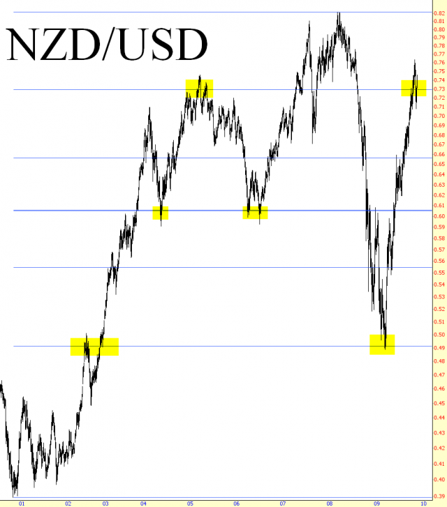
(FIGURE FR-1: There are six major turning points shown here)
Example: Major Market Index
The retracement levels in Figure FR-2 are defined by connecting the low price of July 16, 1996 to the high price of October 15, 2007. Following the establishment of the high price point, the 78.6% retracement served as strong support as the market was weakening in 2008. There were three major instances where the price threatened to break this level but did not.
For the entire period June 6 through September 19, 2008, prices clung to that line level strongly, until at last late in September they fell hard through the 61.8% level, the 50% level, and then finally got support at the 38.2% level. Prices bounced for weeks between the 38.2% and 50% levels until on February 13, 2009, prices made their final plunge to the 23.6% level.
The value at 23.6% is $748.88, and the lowest low that the market reached was $739.29, an almost exact match at 99%. The market bounced hard off this level, barely pausing to rest until it reached the 78.6% retracement line – again, with alarming accuracy. The value of this line is 1240.66, and the index reversed after peaking at 1241.41, which is virtually perfect.
As you can see, the value of retracement levels is to anticipate major turning points. Sometimes the price data pauses (or stops hard) at each level, and other times it will sail through to a subsequent level if the price is too strong or weak to rest at the current station.
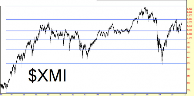
(FIGURE FR-2: The low price in 2009 was anticipated by a fraction of one percent by the Fibonacci retracements of the Major Market Index)
Date of Low Price: 7/16/1996
Date of High Price: 10/15/2007
Example: Nordstrom
A close-up view of retailer Nordstrom’s chart is shown in FR-3. In any of these examples, the thing to focus on before the second date point is how many instances of “bounces” there are between the first and second dates, and the thing to focus on after the second data point is how you might have made use of the retracement levels in your own trading.
In other words, the retracement levels did not exist until such time as the second date. It is interesting to look backwards and notice how and when different bounces off support and resistance took place, but the reality is that the retracement levels would not have been there. However, once the Fibonacci retracement is laid down, examining these touchpoints is useful, because it indicates just how reliable these lines are with respect to the price movement.
If there are many touchpoints, and the lines do seem to have an important relationship with the price movement, then you can have a certain degree of confidence that there will be forthcoming value from these same lines, and in the course of examining these examples, you should reflect on how you would have made use of such lines in your trading.
Turning our attention back to Nordstrom, you can see the price shot up to the first retracement level, paused briefly, continued its ascent to the second level, eased back down to the first, blasted higher to the third level, eased back to the second, and then shot higher to the fourth level. In other words, the classic tendency of a stock to go through a series of “backing and filling” with respect to price is shown here, but it is doing so with a special respect for the levels established by that Fibonacci retracement values.
Therefore, in your own trading, you would have found the best buying opportunities at the points where the price retraced back to a lower price level, and, if you wanted to be conservative and take smaller profits, you would have done well to have taken those profits at the points where the price was at the underside of a retracement level. From this chart, you would have something like:
April 2, 2009- buy
May 7 – sell
June 23 – buy
July 23 – sell
August 19 – buy
September 16 – sell
And all of these decisions would have been based on nothing more than the simple horizontal lines on your screen.
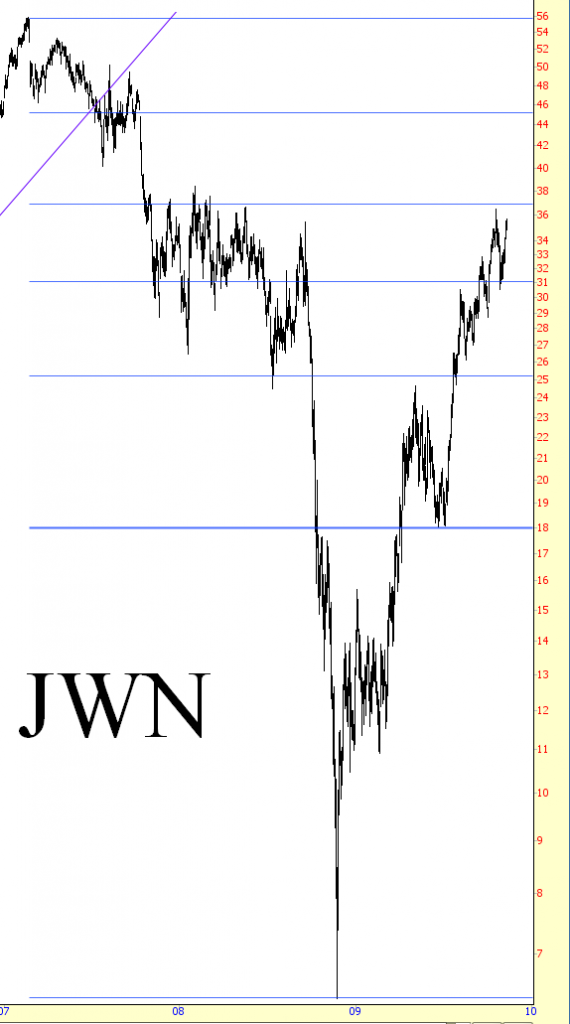
(FIGURE FR-3: Clusters of activity spanning weeks are confined between the retracement levels)
Date of Low Price: 2/22/2007
Date of High Price: 11/21/2008
Example: American Express
Similar to the Nordstrom example, Figure FR-4 shows American Express performing the same “backing and filling”, moving toward, and then away from, each of the retracement levels.
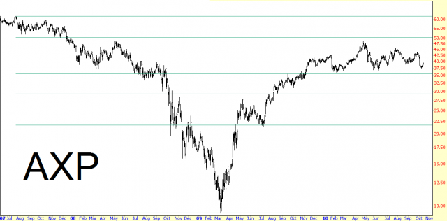
(FIGURE FR-4: The price recovery of 2009 followed a steady path, ascending to one retracement level, backing away to the one just below, and then repeating the process)
Date of Low Price: 7/19/2007
Date of High Price: 3/6/2009
Example: General Electric
The importance of these horizontal lines can even be seen with retracements that span a very long period (in some cases, even as long as a century). General Electric, charted in FR-5, is enhanced with a Fibonacci retracement of about nine years. After GE fell from its peak in 2007 of $36.70 to $5.40 in March 2009 – – an astonishing 86% drop from one of the largest corporations in the world – it began to climb back.
What is remarkable is that the price rose in 2011 to $20.74, which is circled, and the retracement level at this point was $20.61, a difference of merely thirteen cents. Prices are certainly not guaranteed to stop hard at the exactly point where a line is, but they certain can come very close with charts that are conforming to the support and resistance levels suggested by these retracements.
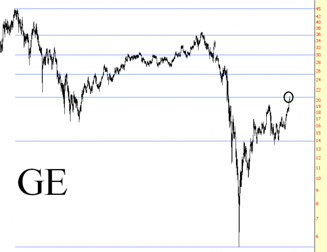
(FIGURE FR-5: The peak price in 2011 seems to have been anticipated in advance by the retracement levels defined by the 2000 and 2009 price extremes)
Date of Low Price: 8/25/2000
Date of High Price: 3/4/2009
Example: Dow Jones Industrials
The Dow Jones Industrial Average has exhibited some very interest behavior with respect to Fibonacci Retracements, only one of which is shown in FR-6. Even very large price ranges – for example, from December 9, 1974 to October 11, 2007 – – provide remarkable instances in which the price is bound (for years at a time in some cases) between two price levels or, conversely, clings tightly to a single price level before shifting to another.
It is worthwhile to experiment with multiple retracements, particularly with an index as long-lived as the Dow 30, to see what kinds of major turning points were pinpointed by certain retracements. Once you have found these, then you can leave those retracements in place to anticipate future significant price levels.
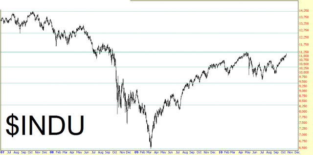
(FIGURE FR-6: The Dow Industrials, the most famous stock index in the world, has exhibited surprisingly reliable behavior toward its retracement levels)
Date of Low Price: 5/7/1996
Date of High Price: 3/6/2009
Example: Lam Research Corporation
Figures FR-7 and and FR-8 show the same stock, Lam Research, but the latter chart shows a close-up view so you can see the price behavior more clearly as it nears various retracement levels.
The timespan for the reference line is large – from 1990 to 2007 – and what happens after the July 2007 data point is interesting and would have been terribly helpful to a person trading this stock from that point forward.
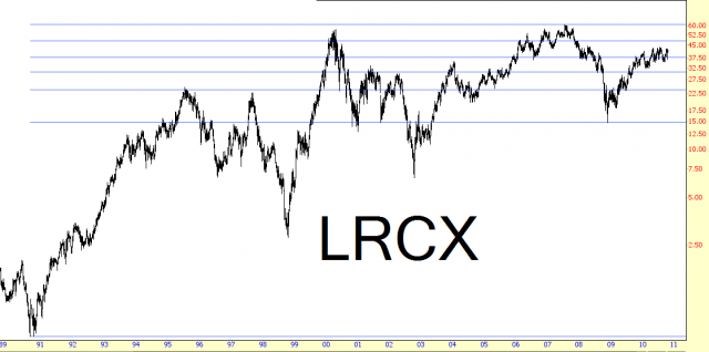
(FIGURE FR-7: The broad, multi-decade view shows many bounces off retracement levels)
The stock starts selling off, and it pauses at the 38.2% level. It continuously bounces at that level from January 9 through July 2 of 2008 before falling next, almost to the penny, to the 50% level. It bounces back up to the 38.2% level and then falls hard down to almost the 78.6% level, at which time it begins a steady ascent, pausing each time it reaches the next lever higher.
When you are looking at a stock chart against these lines, it seems almost predictable and easy, but temporarily remove these lines (which you can do in SlopeCharts by pressing Ctrl-D) and see what a difference it makes. One who becomes accustomed to the guidance Fibonacci retracements can provide may feel they are “flying blind” once those lines disappear, because without them, there’s rarely any clear indication as to where a price may stop rising or falling.
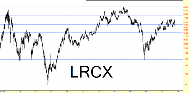
(FIGURE FR-8: This closer view shows that the low price in 2008 was predicted almost to the penny with retracement levels)
Date of Low Price: 8/24/1990
Date of High Price: 7/17/2007
Summary
Retracements are easy to use, because you can focus your attention on a stock only when its price approaches one of those levels. A given level might compel you to buy a stock, short a stock, or take profits on an existing position.
The real challenge comes in identifying the charts that are the best candidates for these retracement levels and taking the right action when those levels are reached (or breached). Given the choice, though, of trading with Fibonacci retracements or without them, you will probably find it much easier (and hopefully more profitable) to have them in your trading arsenal. Used properly, they can be the trader’s equivalent of x-ray vision into the market’s next move.
